Getting Started

[1]:

## SORA package
from sora import Occultation, Body, Star, LightCurve, Observer
from sora.prediction import prediction
from sora.extra import draw_ellipse

## Other main packages
from astropy.time import Time
import astropy.units as u

## Usual packages
import numpy as np
import matplotlib.pylab as pl
import os

SORA version: 1.0dev

Before analysing stellar occultations data, let’s predict them.

To predict stellar occultation we needs the intended Solar System body ephemeris and a time window.

[2]:

# First, let's consider an Solar System Body

chariklo = Body(name='Chariklo',
                ephem=['guidelines/input/bsp/Chariklo.bsp', 'guidelines/input/bsp/de438_small.bsp'])

print(chariklo)

Obtaining data for Chariklo from SBDB
###############################################################################
                          10199 Chariklo (1997 CU26)
###############################################################################
Object Orbital Class: Centaur
Spectral Type:
    SMASS: D  [Reference: EAR-A-5-DDR-TAXONOMY-V4.0]
       Relatively featureless spectrum with very steep red slope.
Discovered 1997-Feb-15 by Spacewatch at Kitt Peak

Physical parameters:
Diameter:
    302 +/- 30 km
    Reference: Earth, Moon, and Planets, v. 89, Issue 1, p. 117-134 (2002),
Rotation:
    7.004 +/- 0 h
    Reference: LCDB (Rev. 2021-June); Warner et al., 2009, [Result based on less than full coverage, so that the period may be wrong by 30 percent or so.]  REFERENCE LIST:[Fornasier, S.; Lazzaro, D.; Alvarez-Candal, A.; Snodgrass, C.; et al. (2014) Astron. Astrophys. 568, L11.], [Leiva, R.; Sicardy, B.; Camargo, J.I.B.; Desmars, J.; et al. (2017) Astron. J. 154, A159.]
Absolute Magnitude:
    6.58 +/- 0 mag
    Reference: MPO647128,
Albedo:
    0.045 +/- 0.01
    Reference: Earth, Moon, and Planets, v. 89, Issue 1, p. 117-134 (2002),

Ellipsoid: 151.0 x 151.0 x 151.0

----------- Ephemeris -----------

EphemKernel: CHARIKLO/DE438_SMALL (SPKID=2010199)
Ephem Error: RA*cosDEC: 0.000 arcsec; DEC: 0.000 arcsec
Offset applied: RA*cosDEC: 0.0000 arcsec; DEC: 0.0000 arcsec

[3]:

pred = prediction(body=chariklo, time_beg='2017-06-20',time_end='2017-06-27',mag_lim=16)

pred

Ephemeris was split in 1 parts for better search of stars

Searching occultations in part 1/1
Generating Ephemeris between 2017-06-20 00:00:00.000 and 2017-06-26 23:59:00.000 ...
Downloading stars ...
    5 GaiaDR3 stars downloaded
Identifying occultations ...

2 occultations found.

[3]:

PredictionTable length=2

Epoch	ICRS Star Coord at Epoch	Geocentric Object Position	C/A	P/A	Vel	Dist	G	long	loct	M-G-T	S-G-T	GaiaDR3 Source ID
			arcsec	deg	km / s	AU	mag	deg	hh:mm	deg	deg
object	object	object	float64	float64	float64	float64	float64	float64	str5	float64	float64	str19
2017-06-21 09:57:43.440	18 55 36.17454 -31 31 19.03261	18 55 36.17500 -31 31 19.60516	0.573	179.41	-21.84	14.663	15.254	225	00:56	128	165	6760228702284187264
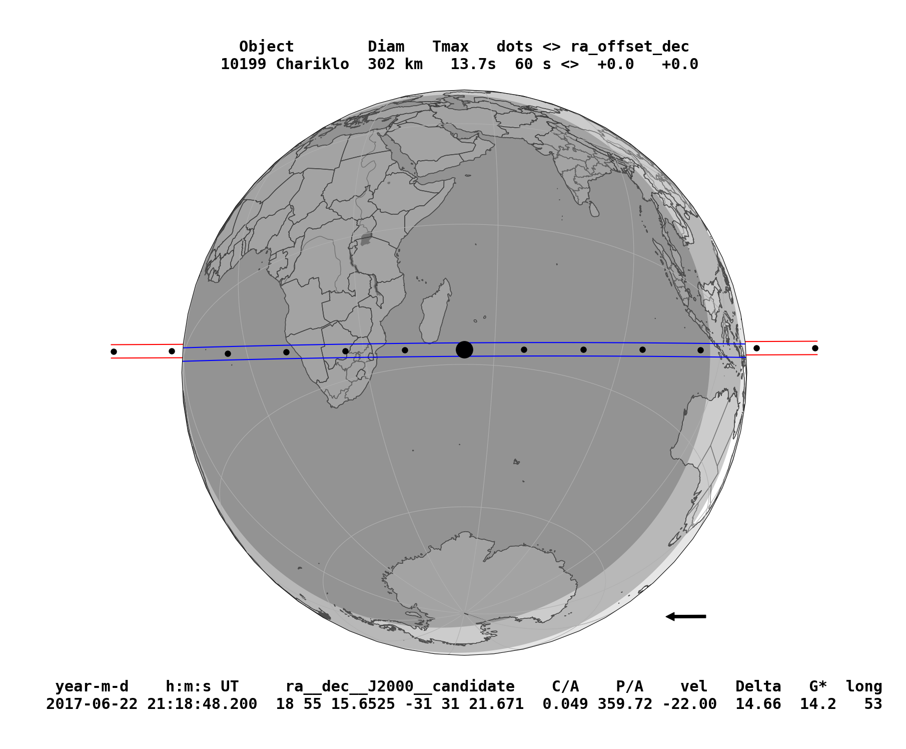
2017-06-22 21:18:48.200	18 55 15.65251 -31 31 21.67062	18 55 15.65249 -31 31 21.62190	0.049	359.72	-22.00	14.659	14.224	53	00:50	149	166	6760223758801661440

[4]:

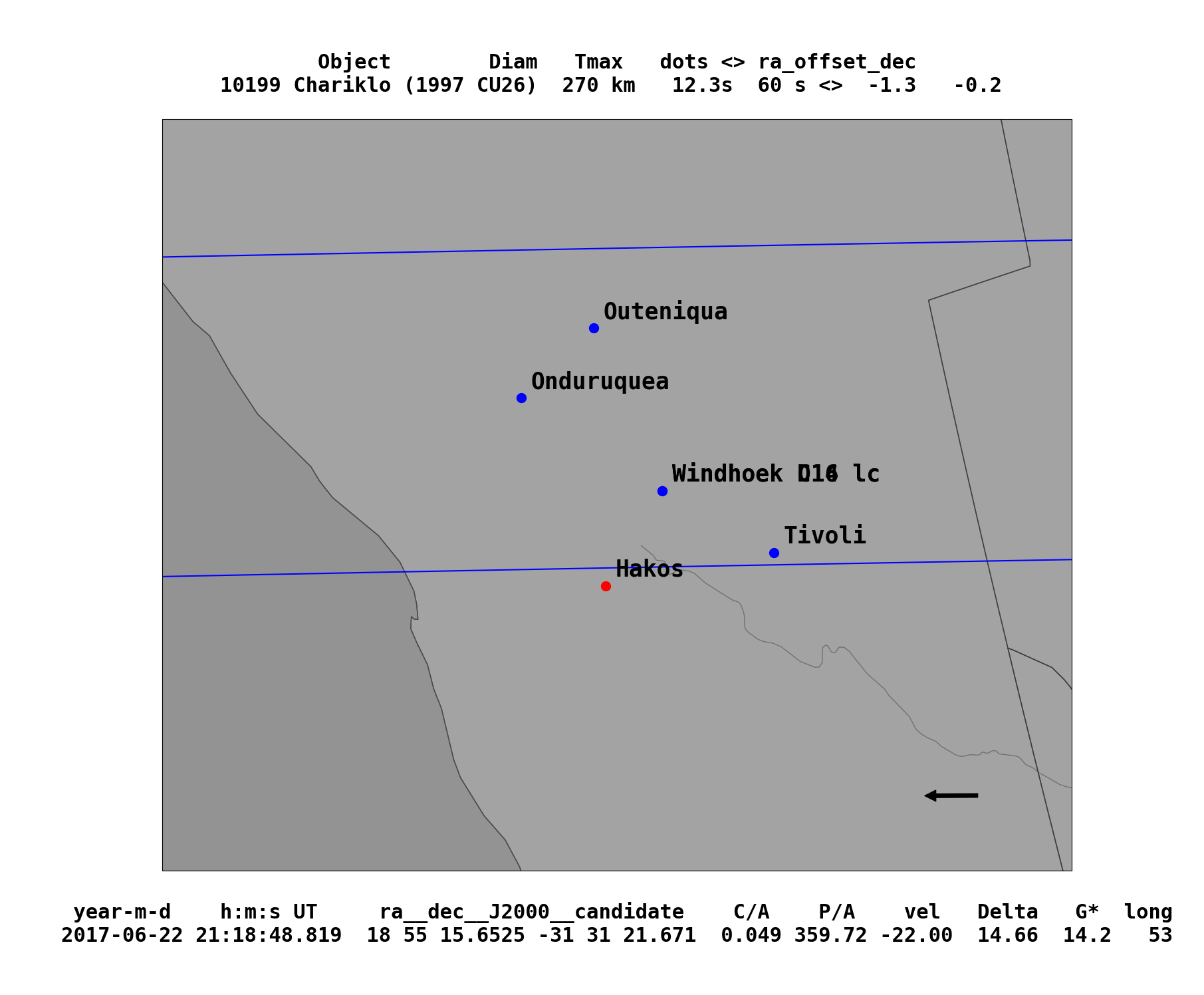
## ploting the occultation map

pred['2017-06-22 21:18'].plot_occ_map(nameimg='guidelines/figures/pred_map')

guidelines/figures/pred_map.png generated

06fcd083f0f8474ab9f9a04d165232b2

Now, let’s start instantiating the Occultation

An occultation is defined by the occulting body, the occulted star, and the time of the occultation

[5]:

Occultation?

Init signature:
Occultation(
    star,
    body=None,
    ephem=None,
    time=None,
    reference_center='geocenter',
)
Docstring:
Instantiates the Occultation object and performs the reduction of the
occultation.

Attributes
----------
star : `sora.Star`, `str`, required
    the coordinate of the star in the same reference frame as the ephemeris.
    It must be a Star object or a string with the coordinates of the object
    to search on Vizier.

body : `sora.Body`, `str`
    Object that will occult the star. It must be a Body object or its name
    to search in the Small Body Database.

ephem : `sora.Ephem`, `list`
    Object ephemeris. It must be an Ephemeris object or a list.

time : `str`, `astropy.time.Time`, required
    Reference time of the occultation. Time does not need to be exact, but
    needs to be within approximately 50 minutes of the occultation closest
    approach to calculate occultation parameters.

reference_center : `str`, `sora.Observer`, `sora.Spacecraft`
    A SORA observer object or a string 'geocenter'.
    The occultation parameters will be calculated in respect
    to this reference as center of projection.


Important
---------
When instantiating with "body" and "ephem", the user may define the
Occultation in 3 ways:

1. With `body` and `ephem`.

2. With only "body". In this case, the "body" parameter must be a Body
object and have an ephemeris associated (see Body documentation).

3. With only `ephem`. In this case, the `ephem` parameter must be one of the
Ephem Classes and have a name (see Ephem documentation) to search for the
body in the Small Body Database.
File:           ~/miniconda3/envs/sora-develop-stats/lib/python3.9/site-packages/sora_astro-1.0.dev0-py3.9.egg/sora/occultation/core.py
Type:           type
Subclasses:

[6]:

star_occ = Star(coord='18 55 15.65250 -31 31 21.67051')
#star_occ = Star(code='6760223758801661440')

print(star_occ)

1 GaiaDR3 star found band={'G': 14.223702}
star coordinate at J2016.0: RA=18h55m15.65210s +/- 0.0197 mas, DEC=-31d31m21.6676s +/- 0.018 mas

Downloading star parameters from I/297/out
GaiaDR3 star Source ID: 6760223758801661440
ICRS star coordinate at J2016.0:
RA=18h55m15.65210s +/- 0.0197 mas, DEC=-31d31m21.6676s +/- 0.0180 mas
pmRA=3.556 +/- 0.025 mas/yr, pmDEC=-2.050 +/- 0.020 mas/yr
GaiaDR3 Proper motion corrected as suggested by Cantat-Gaudin & Brandt (2021)
Plx=0.2121 +/- 0.0228 mas, Rad. Vel.=-40.49 +/- 3.73 km/s

Magnitudes: G: 14.224, B: 14.320, V: 13.530, R: 14.180, J: 12.395, H: 11.781,
            K: 11.627

Apparent diameter from Kervella et. al (2004):
    V: 0.0216 mas, B: 0.0216 mas
Apparent diameter from van Belle (1999):
    sg: B: 0.0238 mas, V: 0.0244 mas
    ms: B: 0.0261 mas, V: 0.0198 mas
    vs: B: 0.0350 mas, V: 0.0315 mas

[7]:

occ = Occultation(star=star_occ, body=chariklo, time='2017-06-22 21:18')

print(occ)

Stellar occultation of star GaiaDR3 6760223758801661440 by 10199 Chariklo (1997 CU26).

Geocentric Closest Approach: 0.049 arcsec
Instant of CA: 2017-06-22 21:18:48.200
Position Angle: 359.72 deg
Geocentric shadow velocity: -22.00 km / s
Sun-Geocenter-Target angle:  166.42 deg
Moon-Geocenter-Target angle: 149.11 deg


No observations reported

###############################################################################
                                     STAR
###############################################################################
GaiaDR3 star Source ID: 6760223758801661440
ICRS star coordinate at J2016.0:
RA=18h55m15.65210s +/- 0.0197 mas, DEC=-31d31m21.6676s +/- 0.0180 mas
pmRA=3.556 +/- 0.025 mas/yr, pmDEC=-2.050 +/- 0.020 mas/yr
GaiaDR3 Proper motion corrected as suggested by Cantat-Gaudin & Brandt (2021)
Plx=0.2121 +/- 0.0228 mas, Rad. Vel.=-40.49 +/- 3.73 km/s

Magnitudes: G: 14.224, B: 14.320, V: 13.530, R: 14.180, J: 12.395, H: 11.781,
            K: 11.627

Apparent diameter from Kervella et. al (2004):
    V: 0.0216 mas, B: 0.0216 mas
Apparent diameter from van Belle (1999):
    sg: B: 0.0238 mas, V: 0.0244 mas
    ms: B: 0.0261 mas, V: 0.0198 mas
    vs: B: 0.0350 mas, V: 0.0315 mas

Geocentric star coordinate at occultation Epoch (2017-06-22 21:18:48.200):
RA=18h55m15.65251s +/- 0.0323 mas, DEC=-31d31m21.6706s +/- 0.0341 mas

###############################################################################
                          10199 Chariklo (1997 CU26)
###############################################################################
Object Orbital Class: Centaur
Spectral Type:
    SMASS: D  [Reference: EAR-A-5-DDR-TAXONOMY-V4.0]
       Relatively featureless spectrum with very steep red slope.
Discovered 1997-Feb-15 by Spacewatch at Kitt Peak

Physical parameters:
Diameter:
    302 +/- 30 km
    Reference: Earth, Moon, and Planets, v. 89, Issue 1, p. 117-134 (2002),
Rotation:
    7.004 +/- 0 h
    Reference: LCDB (Rev. 2021-June); Warner et al., 2009, [Result based on less than full coverage, so that the period may be wrong by 30 percent or so.]  REFERENCE LIST:[Fornasier, S.; Lazzaro, D.; Alvarez-Candal, A.; Snodgrass, C.; et al. (2014) Astron. Astrophys. 568, L11.], [Leiva, R.; Sicardy, B.; Camargo, J.I.B.; Desmars, J.; et al. (2017) Astron. J. 154, A159.]
Absolute Magnitude:
    6.58 +/- 0 mag
    Reference: MPO647128,
Albedo:
    0.045 +/- 0.01
    Reference: Earth, Moon, and Planets, v. 89, Issue 1, p. 117-134 (2002),

Ellipsoid: 151.0 x 151.0 x 151.0

----------- Ephemeris -----------

EphemKernel: CHARIKLO/DE438_SMALL (SPKID=2010199)
Ephem Error: RA*cosDEC: 0.000 arcsec; DEC: 0.000 arcsec
Offset applied: RA*cosDEC: 0.0000 arcsec; DEC: 0.0000 arcsec

After that, we instantiate the observers and their light curves

Observers

Now let’s define our observers, they can be setted manually or from the MPC database

[8]:

### User

out = Observer(name='Outeniqua'  ,lon='+16 49 17.710', lat='-21 17 58.170', height =1416)
ond = Observer(name='Onduruquea' ,lon='+15 59 33.750', lat='-21 36 26.040', height =1220)
tiv = Observer(name='Tivoli'     ,lon='+18 01 01.240', lat='-23 27 40.190', height =1344)
whc = Observer(name='Windhoek'   ,lon='+17 06 31.900', lat='-22 41 55.160', height =1902)
hak = Observer(name='Hakos'      ,lon='+16 21 41.320', lat='-23 14 11.040', height =1843)

print(tiv)

print('\n')

### MPC Database Search

opd = Observer(name='Observatorio Pico dos Dias',code='874')

print(opd)

Site: Tivoli
Geodetic coordinates: Lon: 18d01m01.24s, Lat: -23d27m40.19s, height: 1.344 km


Site: Observatorio Pico dos Dias
Geodetic coordinates: Lon: -45d34m57.54s, Lat: -22d32m07.74756091s, height: 1.811 km

Light Curves

Now let’s define our light curves, they can be instanciated from different way: - (i) Manually with arrays containing the flux and the times; - (ii) Read an ASCII file; - (iii) Already obtained times.

Outeniqua (Namibia)

[9]:

out_lc = LightCurve(name='Outeniqua lc',file='guidelines/input/lightcurves/lc_example.dat',
                    exptime=0.100, usecols=[0,1])

print(out_lc)

Light curve name: Outeniqua lc
Initial time: 2017-06-22 21:20:00.056 UTC
End time:     2017-06-22 21:23:19.958 UTC
Duration:     3.332 minutes
Time offset:  0.000 seconds

Exposure time:    0.1000 seconds
Cycle time:       0.1002 seconds
Num. data points: 2000


There is no occultation associated with this light curve.

Object LightCurve model was not fitted.

Immersion and emersion times were not fitted or instantiated.

[10]:

out_lc.plot_lc()
pl.xlim(76825,76950)
pl.show()

The light curve occultation model considers some physical parameters from the event: - Distance between the geocenter and the occulting object (AU); - Star diameter at the occulting object’s distance (km); - Nominal Velocity of the event (km/s);

These parameters can be automatic calculated as we connect the LightCurve and the Observer to the Ocultation Object.

[11]:

occ.chords.add_chord(observer=out,lightcurve=out_lc)

print(out_lc)

Light curve name: Outeniqua lc
Initial time: 2017-06-22 21:20:00.056 UTC
End time:     2017-06-22 21:23:19.958 UTC
Duration:     3.332 minutes
Time offset:  0.000 seconds

Exposure time:    0.1000 seconds
Cycle time:       0.1002 seconds
Num. data points: 2000

Bandpass:             0.700 +/- 0.300 microns
Object Distance:      14.66 AU
Used shadow velocity: 22.004 km/s
Fresnel scale:        0.040 seconds or 0.87 km
Stellar size effect:  0.010 seconds or 0.23 km

Object LightCurve model was not fitted.

Immersion and emersion times were not fitted or instantiated.

/home/rcboufleur/miniconda3/envs/sora-develop-stats/lib/python3.9/site-packages/sora_astro-1.0.dev0-py3.9.egg/sora/body/core.py:332: UserWarning: H and/or G is not defined for 10199 Chariklo. Searching into JPL Horizons service

Now, appart from the LightCurve Object having the needed parameters, also the Occultation object can acess the information from this Chord.

[12]:

print(occ.chords)

-------------------------------------------------------------------------------
Site: Outeniqua
Geodetic coordinates: Lon: 16d49m17.71s, Lat: -21d17m58.17s, height: 1.416 km
Target altitude: 56.7 deg
Target azimuth:  115.3 deg

Light curve name: Outeniqua lc
Initial time: 2017-06-22 21:20:00.056 UTC
End time:     2017-06-22 21:23:19.958 UTC
Duration:     3.332 minutes
Time offset:  0.000 seconds

Exposure time:    0.1000 seconds
Cycle time:       0.1002 seconds
Num. data points: 2000

Bandpass:             0.700 +/- 0.300 microns
Object Distance:      14.66 AU
Used shadow velocity: 22.004 km/s
Fresnel scale:        0.040 seconds or 0.87 km
Stellar size effect:  0.010 seconds or 0.23 km

Object LightCurve model was not fitted.

Immersion and emersion times were not fitted or instantiated.

[13]:

## We fit the modelled light curve, using chi square minimization and Monte Carlo procedures

out_lc.occ_lcfit?

Signature: out_lc.occ_lcfit(**kwargs)
Docstring:
Monte Carlo chi square fit for occultations lightcurve.

Parameters
----------
tmin : `int`, `float`
    Minimum time to consider in the fit procedure, in seconds.

tmax : `int`, `float`
    Maximum time to consider in the fit procedure, in seconds.

flux_min : `int`, `float`, default=0
    Bottom flux (only object).

flux_max :`int`, `float`, default=1
    Base flux (object plus star).

immersion_time : `int`, `float`
    Initial guess for immersion time, in seconds.

emersion_time : `int`, `float`
    Initial guess for emersion time, in seconds.

opacity : `int`, `float`, default=1
    Initial guess for opacity. Opaque = 1, Transparent = 0.

delta_t : `int`, `float`
    Interval to fit immersion or emersion time.

dopacity : `int`, `float`, default=0
    Interval to fit opacity.

sigma : `int`, `float`, `array`, 'auto'
    Fluxes errors. If None it will use the `self.dflux`. If 'auto' it
    will calculate using the region outside the event.

loop : `int`, default=10000
    Number of tests to be done.

sigma_result : `int`, `float`
    Sigma value to be considered as result.

method : `str`, default=`chisqr`
    Method used to perform the fit. Available methods are:
    `chisqr` : monte carlo computation method used in versions of SORA <= 0.2.1.
    `fastchi` : monte carlo computation method, allows multithreading.
    `least_squares` or `ls`: best fit done used levenberg marquardt convergence algorithm.
    `differential_evolution` or `de`: best fit done using genetic algorithms.
    All methods return a Chisquare object.

threads : `int`
    Number of threads/workers used to perform parallel computations of the chi square
    object. It works with all methods except `chisqr`, by default 1.

Returns
-------
chi2 : `sora.extra.ChiSquare`
    ChiSquare object.
File:      ~/miniconda3/envs/sora-develop-stats/lib/python3.9/site-packages/sora_astro-1.0.dev0-py3.9.egg/sora/lightcurve/core.py
Type:      method

[14]:

## An automatic version can be used for cases where the occultation is obvious!!
## This process may take some minutes to run!!

out_chi2 = out_lc.occ_lcfit(loop=1000)
print('\n')
print(out_chi2)

LightCurve fit: |████████████████████████████████████████|  - 100%


Minimum chi-square: 473.931
Number of fitted points: 496
Number of fitted parameters: 2
Minimum chi-square per degree of freedom: 0.959

immersion:
    1-sigma: 76880.322 +/- 0.032
    3-sigma: 76880.353 +/- 0.131

emersion:
    1-sigma: 76890.349 +/- 0.031
    3-sigma: 76890.347 +/- 0.108

[15]:

## However, we believe that the user should set the parameters by hand!!
## The complete description of each parameter can be seen at the function Docstring.
## This process may take some minutes to run!!

out_chi2 = out_lc.occ_lcfit(tmin=76875.0, tmax=76895.0,
                            immersion_time=76880.3,
                            emersion_time=76890.3,
                            delta_t=0.2, loop=10000)
print('\n')
print(out_chi2)

LightCurve fit: |████████████████████████████████████████|  - 100%


Minimum chi-square: 192.774
Number of fitted points: 200
Number of fitted parameters: 2
Minimum chi-square per degree of freedom: 0.974

immersion:
    1-sigma: 76880.325 +/- 0.027
    3-sigma: 76880.347 +/- 0.121

emersion:
    1-sigma: 76890.351 +/- 0.029
    3-sigma: 76890.348 +/- 0.101

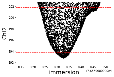
The user can visually acess the quality of the fit by ploting the ChiSquare object.

[16]:

out_chi2.plot_chi2('immersion')
pl.xlim(76880.33 - 0.20, 76880.33 + 0.20)
pl.show()

out_chi2.plot_chi2('emersion')
pl.xlim(76890.34 - 0.20, 76890.34 + 0.20)
pl.show()

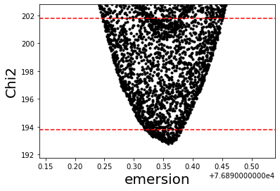
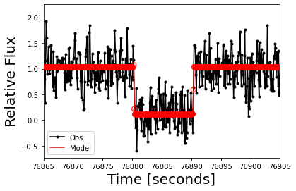
Also, the user can visually acess the quality of the fit by ploting the LightCurve.

[17]:

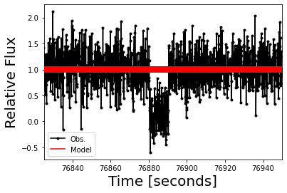
out_lc.plot_lc()
pl.xlim(76865, 76905)
pl.show()

out_lc.plot_model()
pl.xlim(76890.34-0.5, 76890.34+0.5)
pl.legend(ncol=1, fontsize=12.5, loc=2)
pl.show()

[18]:

print(out_lc)

Light curve name: Outeniqua lc
Initial time: 2017-06-22 21:20:00.056 UTC
End time:     2017-06-22 21:23:19.958 UTC
Duration:     3.332 minutes
Time offset:  0.000 seconds

Exposure time:    0.1000 seconds
Cycle time:       0.1002 seconds
Num. data points: 2000

Bandpass:             0.700 +/- 0.300 microns
Object Distance:      14.66 AU
Used shadow velocity: 22.004 km/s
Fresnel scale:        0.040 seconds or 0.87 km
Stellar size effect:  0.010 seconds or 0.23 km
Inst. response:       0.100 seconds or 2.20 km
Dead time effect:     0.000 seconds or 0.00 km
Model resolution:     0.004 seconds or 0.09 km
Modelled baseflux:    1.029
Modelled bottomflux:  0.109
Light curve sigma:    0.307

Immersion time: 2017-06-22 21:21:20.325 UTC +/- 0.027 seconds
Emersion time:  2017-06-22 21:21:30.351 UTC +/- 0.029 seconds

Monte Carlo chi square fit.

Minimum chi-square: 192.774
Number of fitted points: 200
Number of fitted parameters: 2
Minimum chi-square per degree of freedom: 0.974

immersion:
    1-sigma: 76880.325 +/- 0.027
    3-sigma: 76880.347 +/- 0.121

emersion:
    1-sigma: 76890.351 +/- 0.029
    3-sigma: 76890.348 +/- 0.101

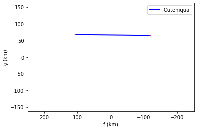
Finally, the user can visually see the chord in the Sky-plane using the Chord Object.

[19]:

occ.chords.plot_chords(segment='positive', color='blue')
occ.chords.plot_chords(segment='error', color='red')
pl.legend()
pl.xlim(+250,-250)
pl.ylim(-250,+250)
pl.show()

Now, let’s add the other chords of this occultation.

Onduruquea (Namibia)

[20]:

ond_lc = LightCurve(name='Onduruquea lc',
                    initial_time='2017-06-22 21:11:52.175',
                    end_time ='2017-06-22 21:25:13.389',
                    immersion='2017-06-22 21:21:22.213', immersion_err=0.010,
                    emersion ='2017-06-22 21:21:33.824', emersion_err=0.011)

occ.chords.add_chord(observer=ond,lightcurve=ond_lc)

[20]:

<Chord: Onduruquea>

[21]:

print(occ.chords['Onduruquea'])

-------------------------------------------------------------------------------
Site: Onduruquea
Geodetic coordinates: Lon: 15d59m33.75s, Lat: -21d36m26.04s, height: 1.220 km
Target altitude: 56.1 deg
Target azimuth:  114.7 deg

Light curve name: Onduruquea lc
Initial time: 2017-06-22 21:11:52.175 UTC
End time:     2017-06-22 21:25:13.389 UTC
Duration:     13.354 minutes
Time offset:  0.000 seconds

Object LightCurve was not instantiated with time and flux.

Bandpass:             0.700 +/- 0.300 microns
Object Distance:      14.66 AU
Used shadow velocity: 22.004 km/s
Fresnel scale:        0.040 seconds or 0.87 km
Stellar size effect:  0.010 seconds or 0.23 km

Object LightCurve model was not fitted.

Immersion time: 2017-06-22 21:21:22.213 UTC +/- 0.010 seconds
Emersion time:  2017-06-22 21:21:33.824 UTC +/- 0.011 seconds

Tivoli (Namibia)

[22]:

tiv_lc = LightCurve(name='Tivoli lc',
                    initial_time='2017-06-22 21:16:00.094',
                    end_time ='2017-06-22 21:28:00.018',
                    immersion='2017-06-22 21:21:15.628',immersion_err=0.011,
                    emersion ='2017-06-22 21:21:19.988',emersion_err=0.038)

occ.chords.add_chord(observer=tiv, lightcurve=tiv_lc)

[22]:

<Chord: Tivoli>

Windhoek (Namibia)

When there is two chords at the same stations is important to define their names as different values

[23]:

## C14
whc_c14_lc = LightCurve(name='Windhoek C14 lc',
                    initial_time='2017-06-22 21:12:48.250',
                    end_time ='2017-06-22 21:32:47.963',
                    immersion='2017-06-22 21:21:17.609',immersion_err=0.024,
                    emersion ='2017-06-22 21:21:27.564',emersion_err=0.026)

occ.chords.add_chord(name='Windhoek C14 lc', observer=whc, lightcurve=whc_c14_lc)

## D16
whc_d16_lc = LightCurve(name='Windhoek D16 lc',
                    initial_time='2017-06-22 21:20:01.884',
                    end_time ='2017-06-22 21:22:21.894',
                    immersion='2017-06-22 21:21:17.288',immersion_err=0.028,
                    emersion ='2017-06-22 21:21:27.228',emersion_err=0.034)

occ.chords.add_chord(name='Windhoek D16 lc', observer=whc, lightcurve=whc_d16_lc)

[23]:

<Chord: Windhoek D16 lc>

Hakos (Namibia)

[24]:

#Also negatives chords can be added
hak_lc = LightCurve(name='Hakos lc',
                    initial_time='2017-06-22 21:10:19.461',
                    end_time ='2017-06-22 21:30:19.345')

occ.chords.add_chord(observer=hak, lightcurve=hak_lc)

[24]:

<Chord: Hakos>

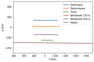
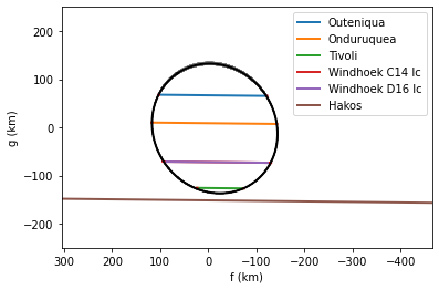
Chords display and ellipse fit

After all light curves were instanciated and/or fitted, the next step is to plot the chords and fit the elipse.

[25]:

occ.chords.plot_chords()
occ.chords.plot_chords(segment='error', color='red')

pl.legend(loc=1)
pl.xlim(+170,-330)
pl.ylim(-250,+250)
pl.show()

[26]:

## We can add known time offsets due to camera features

out_lc.dt = -0.150
ond_lc.dt = -0.190
tiv_lc.dt = -0.150
whc_c14_lc.dt = -0.375
whc_d16_lc.dt = +0.000
hak_lc.dt = -0.200

[27]:

occ.chords.plot_chords()
occ.chords.plot_chords(segment='error', color='red')

pl.legend(loc=1)
pl.xlim(+170,-330)
pl.ylim(-250,+250)
pl.show()

The next step is to fit an ellipse to the chords

[28]:

## We fit a ellipse using chi square minimization and Monte Carlo procedures, the
## The complete description of each parameter can be seen at the function Docstring.

occ.fit_ellipse?

Signature: occ.fit_ellipse(**kwargs)
Docstring:
Fits an ellipse to given occultation using given parameters.

Parameters
----------
center_f : `int`, `float`, default=0
    The coordinate in f of the ellipse center.

center_g : `int`, `float`, default=0
    The coordinate in g of the ellipse center.

equatorial_radius : `int`, `float`
    The Equatorial radius (semi-major axis) of the ellipse.

oblateness : `int`, `float`, default=0
    The oblateness of the ellipse.

position_angle : `int`, `float`, default=0
    The pole position angle of the ellipse in degrees.
    Zero is in the North direction ('g-positive'). Positive clockwise.

dcenter_f : `int`, `float`
    Interval for coordinate f of the ellipse center.

dcenter_g : `int`, `float`
    Interval for coordinate g of the ellipse center.

dequatorial_radius `int`, `float`
    Interval for the Equatorial radius (semi-major axis) of the ellipse.

doblateness : `int`, `float`
    Interval for the oblateness of the ellipse

dposition_angle : `int`, `float`
    Interval for the pole position angle of the ellipse in degrees.

loop : `int`, default=10000000
    The number of ellipses to attempt fitting.

dchi_min : `int`, `float`
    If given, it will only save ellipsis which chi square are smaller than
    chi_min + dchi_min. By default `None` when used with `method='chisqr`, and
    `3` for other methods.

number_chi : `int`, default=10000
    In the `chisqr` method if `dchi_min` is given, the procedure is repeated until
    `number_chi` is reached.
    In other methods it is the number of values (simulations) that should lie within
    the provided `sigma_result`.

verbose : `bool`, default=False
    If True, it prints information while fitting.

ellipse_error : `int`, `float`
    Model uncertainty to be considered in the fit, in km.

sigma_result : `int`, `float`
    Sigma value to be considered as result.

method : `str`, default=`least_squares`
    Method used to perform the fit. Available methods are:
    `chisqr` : monte carlo computation method used in versions of SORA <= 0.2.1.
    `fastchi` : monte carlo computation method, allows multithreading .
    `least_squares` or `ls`: best fit done used levenberg marquardt convergence algorithm.
    `differential_evolution` or ``de`: best fit done using genetic algorithms.
    All methods return a Chisquare object.

threads : `int`
    Number of threads/workers used to perform parallel computations of the chi square
    object. It works with all methods except `chisqr`, by default 1.

Returns
-------
chisquare : `sora.ChiSquare`
    A ChiSquare object with all parameters.

Important
---------
Each occultation is added as the first argument(s) directly.

Mandatory input parameters: 'center_f', 'center_g', 'equatorial_radius',
'oblateness', and 'position_angle'.

Parameters fitting interval: 'dcenter_f', 'dcenter_g', 'dequatorial_radius',
'doblateness', and 'dposition_angle'. Default values are set to zero.
Search done between (value - dvalue) and (value + dvalue).


Examples
--------
To fit the ellipse to the chords of occ1 Occultation object:

>>> fit_ellipse(occ1, **kwargs)

To fit the ellipse to the chords of occ1 and occ2 Occultation objects together:

>>> fit_ellipse(occ1, occ2, **kwargs)
File:      ~/miniconda3/envs/sora-develop-stats/lib/python3.9/site-packages/sora_astro-1.0.dev0-py3.9.egg/sora/occultation/core.py
Type:      method

[29]:

### This may take some minutes to run!!

ellipse_chi2  = occ.fit_ellipse(center_f=-15.046, center_g=-2.495, dcenter_f=3, dcenter_g=10,
                                equatorial_radius=138, dequatorial_radius=3, oblateness=0.093,
                                doblateness=0.02, position_angle=126, dposition_angle=10 ,loop=10000000,
                                dchi_min=10,number_chi=10000)


print(ellipse_chi2)

Minimum chi-square: 12.130
Number of fitted points: 10
Number of fitted parameters: 5
Minimum chi-square per degree of freedom: 2.426

center_f:
    1-sigma: -13.613 +/- 0.120
    3-sigma: -13.611 +/- 0.430

center_g:
    1-sigma: -2.094 +/- 0.499
    3-sigma: -2.089 +/- 1.626

equatorial_radius:
    1-sigma: 138.657 +/- 0.373
    3-sigma: 138.673 +/- 1.445

oblateness:
    1-sigma: 0.086 +/- 0.003
    3-sigma: 0.086 +/- 0.010

position_angle:
    1-sigma: 123.956 +/- 1.496
    3-sigma: 124.121 +/- 5.140

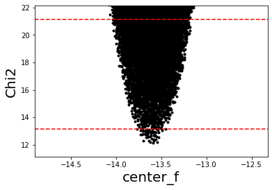
Similar, to the LightCurve fit, the user can visually acess the quality of the fit by ploting the ChiSquare object.

[30]:

ellipse_chi2.plot_chi2()

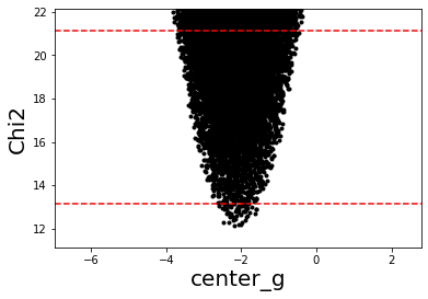
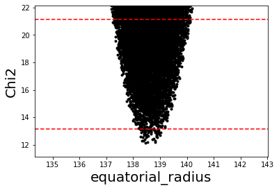
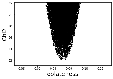
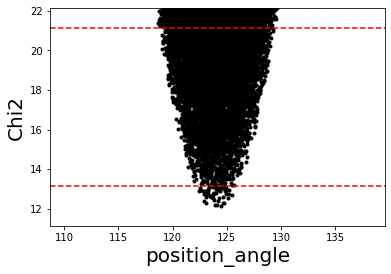
Also, the user can visually acess the quality of the fit by ploting the Chords and the fitted ellipses.

[31]:

occ.chords.plot_chords()
occ.chords.plot_chords(segment='error', color='red')

#plotting the best fitted ellipse, in black
draw_ellipse(**ellipse_chi2.get_values())

# ploting all the ellipses within 3-sigma, in gray
draw_ellipse(**ellipse_chi2.get_values(sigma=3),alpha=1.0)

pl.legend(loc=1)
pl.xlim(+170,-330)
pl.ylim(-250,+250)
pl.show()

The resulting values can be acessed from the Dictionaries Occultation.fitted_params and Occultation.chi2_params

[32]:

occ.fitted_params

[32]:

{'equatorial_radius': [138.65650796361007, 0.3729805506807651],
 'center_f': [-13.612927096827903, 0.11996518649955146],
 'center_g': [-2.0936385736495167, 0.4992405703706848],
 'oblateness': [0.08573692161473534, 0.003305360393147015],
 'position_angle': [123.95618703950413, 1.4957816035600828]}

[33]:

occ.chi2_params

[33]:

{'chord_name': ['Outeniqua_immersion',
  'Outeniqua_emersion',
  'Onduruquea_immersion',
  'Onduruquea_emersion',
  'Tivoli_immersion',
  'Tivoli_emersion',
  'Windhoek C14 lc_immersion',
  'Windhoek C14 lc_emersion',
  'Windhoek D16 lc_immersion',
  'Windhoek D16 lc_emersion'],
 'radial_dispersion': array([ 0.64886238, -0.82234285, -0.20941195,  0.0507056 ,  0.14404744,
        -2.02271261,  0.3135147 , -0.1926379 , -0.76516855,  0.53220478]),
 'position_angle': array([301.95754708,  58.93979955, 274.10063776,  84.70868609,
        205.80484092, 163.27224646, 238.45346645, 123.09039914,
        238.19141651, 122.87262257]),
 'radial_error': array([0.60995255, 0.64472971, 0.22353256, 0.24588816, 0.24592892,
        0.8495755 , 0.53652931, 0.58124429, 0.62595044, 0.76008871]),
 'chi2_min': 12.129614721820191,
 'nparam': 5,
 'npts': 10}

Besides the size and shape of the body the astrometrical positions obtained using stellar occultation is also a relevant result from the occultation and it has a precision that can be compared with space probes results (few km)

[34]:

occ.new_astrometric_position()

Ephemeris offset (km): X = -13.6 km +/- 0.1 km; Y = -2.1 km +/- 0.5 km
Ephemeris offset (mas): da_cos_dec = -1.280 +/- 0.011; d_dec = -0.197 +/- 0.047

Astrometric object position at time 2017-06-22 21:18:48.200 for reference 'geocenter'
RA = 18 55 15.6523911 +/- 0.034 mas; DEC = -31 31 21.622094 +/- 0.058 mas

After the instanciation of the Chords and the ellipse fit, the posfit occultation map can be plotted.

[35]:

occ.plot_occ_map(centermap_delta=[-3500,+400],zoom=20,nameimg='guidelines/figures/map_posfit')

Projected shadow radius = 135.0 km
guidelines/figures/map_posfit.png generated

7fd30df2413841e1b78ee14faa78c9c2

Finally, the log contains all the details

[36]:

print(occ)

Stellar occultation of star GaiaDR3 6760223758801661440 by 10199 Chariklo (1997 CU26).

Geocentric Closest Approach: 0.049 arcsec
Instant of CA: 2017-06-22 21:18:48.200
Position Angle: 359.72 deg
Geocentric shadow velocity: -22.00 km / s
Sun-Geocenter-Target angle:  166.42 deg
Moon-Geocenter-Target angle: 149.11 deg


5 positive observations
1 negative observations

###############################################################################
                                     STAR
###############################################################################
GaiaDR3 star Source ID: 6760223758801661440
ICRS star coordinate at J2016.0:
RA=18h55m15.65210s +/- 0.0197 mas, DEC=-31d31m21.6676s +/- 0.0180 mas
pmRA=3.556 +/- 0.025 mas/yr, pmDEC=-2.050 +/- 0.020 mas/yr
GaiaDR3 Proper motion corrected as suggested by Cantat-Gaudin & Brandt (2021)
Plx=0.2121 +/- 0.0228 mas, Rad. Vel.=-40.49 +/- 3.73 km/s

Magnitudes: G: 14.224, B: 14.320, V: 13.530, R: 14.180, J: 12.395, H: 11.781,
            K: 11.627

Apparent diameter from Kervella et. al (2004):
    V: 0.0216 mas, B: 0.0216 mas
Apparent diameter from van Belle (1999):
    sg: B: 0.0238 mas, V: 0.0244 mas
    ms: B: 0.0261 mas, V: 0.0198 mas
    vs: B: 0.0350 mas, V: 0.0315 mas

Geocentric star coordinate at occultation Epoch (2017-06-22 21:18:48.200):
RA=18h55m15.65251s +/- 0.0323 mas, DEC=-31d31m21.6706s +/- 0.0341 mas

###############################################################################
                          10199 Chariklo (1997 CU26)
###############################################################################
Object Orbital Class: Centaur
Spectral Type:
    SMASS: D  [Reference: EAR-A-5-DDR-TAXONOMY-V4.0]
       Relatively featureless spectrum with very steep red slope.
Discovered 1997-Feb-15 by Spacewatch at Kitt Peak

Physical parameters:
Diameter:
    302 +/- 30 km
    Reference: Earth, Moon, and Planets, v. 89, Issue 1, p. 117-134 (2002),
Rotation:
    7.004 +/- 0 h
    Reference: LCDB (Rev. 2021-June); Warner et al., 2009, [Result based on less than full coverage, so that the period may be wrong by 30 percent or so.]  REFERENCE LIST:[Fornasier, S.; Lazzaro, D.; Alvarez-Candal, A.; Snodgrass, C.; et al. (2014) Astron. Astrophys. 568, L11.], [Leiva, R.; Sicardy, B.; Camargo, J.I.B.; Desmars, J.; et al. (2017) Astron. J. 154, A159.]
Absolute Magnitude:
    6.58 +/- 0 mag
    Reference: JPL Horizons,
Phase Slope:
    0.15 +/- 0
    Reference: JPL Horizons,
Albedo:
    0.045 +/- 0.01
    Reference: Earth, Moon, and Planets, v. 89, Issue 1, p. 117-134 (2002),

Ellipsoid: 151.0 x 151.0 x 151.0

----------- Ephemeris -----------

EphemKernel: CHARIKLO/DE438_SMALL (SPKID=2010199)
Ephem Error: RA*cosDEC: 0.000 arcsec; DEC: 0.000 arcsec
Offset applied: RA*cosDEC: 0.0000 arcsec; DEC: 0.0000 arcsec


###############################################################################
                             POSITIVE OBSERVATIONS
###############################################################################

-------------------------------------------------------------------------------
Site: Outeniqua
Geodetic coordinates: Lon: 16d49m17.71s, Lat: -21d17m58.17s, height: 1.416 km
Target altitude: 56.6 deg
Target azimuth:  115.3 deg

Light curve name: Outeniqua lc
Initial time: 2017-06-22 21:20:00.056 UTC
End time:     2017-06-22 21:23:19.958 UTC
Duration:     3.332 minutes
Time offset:  -0.150 seconds

Exposure time:    0.1000 seconds
Cycle time:       0.1002 seconds
Num. data points: 2000

Bandpass:             0.700 +/- 0.300 microns
Object Distance:      14.66 AU
Used shadow velocity: 22.004 km/s
Fresnel scale:        0.040 seconds or 0.87 km
Stellar size effect:  0.010 seconds or 0.23 km
Inst. response:       0.100 seconds or 2.20 km
Dead time effect:     0.000 seconds or 0.00 km
Model resolution:     0.004 seconds or 0.09 km
Modelled baseflux:    1.029
Modelled bottomflux:  0.109
Light curve sigma:    0.307

Immersion time: 2017-06-22 21:21:20.175 UTC +/- 0.027 seconds
Emersion time:  2017-06-22 21:21:30.201 UTC +/- 0.029 seconds

Monte Carlo chi square fit.

Minimum chi-square: 192.774
Number of fitted points: 200
Number of fitted parameters: 2
Minimum chi-square per degree of freedom: 0.974

immersion:
    1-sigma: 76880.325 +/- 0.027
    3-sigma: 76880.347 +/- 0.121

emersion:
    1-sigma: 76890.351 +/- 0.029
    3-sigma: 76890.348 +/- 0.101


-------------------------------------------------------------------------------
Site: Onduruquea
Geodetic coordinates: Lon: 15d59m33.75s, Lat: -21d36m26.04s, height: 1.220 km
Target altitude: 56.1 deg
Target azimuth:  114.7 deg

Light curve name: Onduruquea lc
Initial time: 2017-06-22 21:11:52.175 UTC
End time:     2017-06-22 21:25:13.389 UTC
Duration:     13.354 minutes
Time offset:  -0.190 seconds

Object LightCurve was not instantiated with time and flux.

Bandpass:             0.700 +/- 0.300 microns
Object Distance:      14.66 AU
Used shadow velocity: 22.004 km/s
Fresnel scale:        0.040 seconds or 0.87 km
Stellar size effect:  0.010 seconds or 0.23 km

Object LightCurve model was not fitted.

Immersion time: 2017-06-22 21:21:22.023 UTC +/- 0.010 seconds
Emersion time:  2017-06-22 21:21:33.634 UTC +/- 0.011 seconds


-------------------------------------------------------------------------------
Site: Tivoli
Geodetic coordinates: Lon: 18d01m01.24s, Lat: -23d27m40.19s, height: 1.344 km
Target altitude: 58.5 deg
Target azimuth:  112.4 deg

Light curve name: Tivoli lc
Initial time: 2017-06-22 21:16:00.094 UTC
End time:     2017-06-22 21:28:00.018 UTC
Duration:     11.999 minutes
Time offset:  -0.150 seconds

Object LightCurve was not instantiated with time and flux.

Bandpass:             0.700 +/- 0.300 microns
Object Distance:      14.66 AU
Used shadow velocity: 22.004 km/s
Fresnel scale:        0.040 seconds or 0.87 km
Stellar size effect:  0.010 seconds or 0.23 km

Object LightCurve model was not fitted.

Immersion time: 2017-06-22 21:21:15.478 UTC +/- 0.011 seconds
Emersion time:  2017-06-22 21:21:19.838 UTC +/- 0.038 seconds


-------------------------------------------------------------------------------
Site: Windhoek
Geodetic coordinates: Lon: 17d06m31.9s, Lat: -22d41m55.16s, height: 1.902 km
Target altitude: 57.4 deg
Target azimuth:  113.4 deg

Light curve name: Windhoek C14 lc
Initial time: 2017-06-22 21:12:48.250 UTC
End time:     2017-06-22 21:32:47.963 UTC
Duration:     19.995 minutes
Time offset:  -0.375 seconds

Object LightCurve was not instantiated with time and flux.

Bandpass:             0.700 +/- 0.300 microns
Object Distance:      14.66 AU
Used shadow velocity: 22.004 km/s
Fresnel scale:        0.040 seconds or 0.87 km
Stellar size effect:  0.010 seconds or 0.23 km

Object LightCurve model was not fitted.

Immersion time: 2017-06-22 21:21:17.234 UTC +/- 0.024 seconds
Emersion time:  2017-06-22 21:21:27.189 UTC +/- 0.026 seconds


-------------------------------------------------------------------------------
Site: Windhoek
Geodetic coordinates: Lon: 17d06m31.9s, Lat: -22d41m55.16s, height: 1.902 km
Target altitude: 57.4 deg
Target azimuth:  113.4 deg

Light curve name: Windhoek D16 lc
Initial time: 2017-06-22 21:20:01.884 UTC
End time:     2017-06-22 21:22:21.894 UTC
Duration:     2.333 minutes
Time offset:  0.000 seconds

Object LightCurve was not instantiated with time and flux.

Bandpass:             0.700 +/- 0.300 microns
Object Distance:      14.66 AU
Used shadow velocity: 22.004 km/s
Fresnel scale:        0.040 seconds or 0.87 km
Stellar size effect:  0.010 seconds or 0.23 km

Object LightCurve model was not fitted.

Immersion time: 2017-06-22 21:21:17.288 UTC +/- 0.028 seconds
Emersion time:  2017-06-22 21:21:27.228 UTC +/- 0.034 seconds


###############################################################################
                             NEGATIVE OBSERVATIONS
###############################################################################

-------------------------------------------------------------------------------
Site: Hakos
Geodetic coordinates: Lon: 16d21m41.32s, Lat: -23d14m11.04s, height: 1.843 km
Target altitude: 56.8 deg
Target azimuth:  112.5 deg

Light curve name: Hakos lc
Initial time: 2017-06-22 21:10:19.461 UTC
End time:     2017-06-22 21:30:19.345 UTC
Duration:     19.998 minutes
Time offset:  -0.200 seconds

Object LightCurve was not instantiated with time and flux.

Bandpass:             0.700 +/- 0.300 microns
Object Distance:      14.66 AU
Used shadow velocity: 22.004 km/s
Fresnel scale:        0.040 seconds or 0.87 km
Stellar size effect:  0.010 seconds or 0.23 km

Object LightCurve model was not fitted.

Immersion and emersion times were not fitted or instantiated.


###############################################################################
                                    RESULTS
###############################################################################

Fitted Ellipse:
equatorial_radius: 138.657 +/- 0.373
center_f: -13.613 +/- 0.120
center_g: -2.094 +/- 0.499
oblateness: 0.086 +/- 0.003
position_angle: 123.956 +/- 1.496
polar_radius: 126.769 km
equivalent_radius: 132.579 km
geometric albedo (V): 0.060 (6.0%)

Minimum chi-square: 12.130
Number of fitted points: 10
Number of fitted parameters: 5
Minimum chi-square per degree of freedom: 2.426
Radial dispersion: -0.232 +/- 0.797 km
Radial error:      0.532 +/- 0.222 km

Ephemeris offset (km): X = -13.6 km +/- 0.1 km; Y = -2.1 km +/- 0.5 km
Ephemeris offset (mas): da_cos_dec = -1.280 +/- 0.011; d_dec = -0.197 +/- 0.047

Astrometric object position at time 2017-06-22 21:18:48.200 for reference 'geocenter'
RA = 18 55 15.6523911 +/- 0.034 mas; DEC = -31 31 21.622094 +/- 0.058 mas

You can find more information about each Class at their specific Jupyter-Notebook.

The END